CU-4  CU Point Addition Method

Summary

This method describes a mathematical operation on points that lie on a specific cubic curve (CU). Through a geometric construction, a group structure is defined in which two points on the curve are combined to form a third. The CU Point Addition Method forms the core of this structure and provides a consistent way to perform point additions within the domain of the curve, giving rise to numerous applications in which conjectures can be tested and validated.

Historical Context

The method of point addition on elliptic curves originates from Niels Henrik Abel (1802–1829). Abel studied elliptic integrals and discovered that they cannot always be expressed in terms of elementary functions. His work led to the concept of elliptic functions, which were later directly connected to elliptic curves.He introduced the idea of a group structure on curves via analytic functions. Other mathematicians such as Carl Gustav Jacobi (1804–1851), Karl Weierstrass (1815–1897), and Henri Poincaré (1854–1912) expanded the theory.

Fred Lang wrote the article Geometry and Group Structures of Some Cubics, published in Forum Geometricorum, Vol. 2 (2002). Lang generalizes the method for broader classes of cubic curves in the projective plane. Among other things, he introduces a neutral element O.See [77].

What does point addition involve?

On an elliptic curve, two points P and Q can be added as follows:

• Draw a line through P and Q.
• Determine the third intersection point of that line with the curve.
• Reflect that point across the x-axis (in the real plane).
• The result is the point P + Q.

This was the known method.Lang generalizes this approach for broader classes of cubic curves in the projective plane. He introduces a neutral element O and defines the group operation as:

• P + Q = (P . Q) . O

where P . Q is the third intersection point of the line through P and Q, and . O is an additional operation involving the neutral point.

Some notable insights from Lang’s work:

• The operation is commutative, but not always associative without additional conditions.
• He uses this structure to analyze properties of classical cubic curves such as those of Thomson, Darboux, and Lucas.
• Connections are made between collinearity of points and their sum in the group:
  • Three CU-points are collinear ⟺ their sum equals a fixed point N.
  • Six CU-points lie on a conic ⟺ their sum is 2N.
  • Nine CU-points lie on another cubic curve ⟺ their sum is 3N.

It is remarkable how many problems can be solved using these simple rules.

ELABORATION

Definitions and conventions

• Let CU be a nonsingular reference cubic curve without cusp or node in the complex projective plane.
• Let O be some point on CU functioning as Origin.
• Points Pi (P1, P2, P3, etc.) are supposed to be reference points on CU.
• Two operations are used, the . operation and the + operation.
  • P1·P2 is defined as the third intersection of the line P1P2 with CU.
  • P1+P2 is defined as (P1.P2).O
• The + operation defines a group structure on the points on CU, satisfying closure, associativity ((a + b) + c = a + (b + c)), identity and inverse. Here the identity element is 0, and the inverse is the negative. The group is abelian, meaning the operation is also commutative (a + b = b + a).
• The tangential point of a point P is the intersection of CU with the tangent at P.
• Denote the sum P1+P2+ … +Pi by PPi.

Rules for adding points

1. Any point O on a reference cubic CU can be choden as the origin. Let N be the tangential point of O.
2. You can assign values to any point on the cubic. O has value 0 (zero). N has value N, and other points on the cubic are valued bu their name.
3. -P1 = O.P1
4. N-P1-P2 = P1.P2
5. P1+P2 = O.(P1.P2)
6. When P1,P2,P3 on CU are collinear then P1+P2+P3 = N
7. When P1 through P6 on CU are coconic then P1+P2+P3+P4+P5+P6 = 2N
8. When P1 through P9 on CU lie on another cubic, then P1+P2+ … +P9 = 3N
9. For intersection points of CU with curves of degree n (n>3), then P1+ … +Pm=nN, where m=3n.
10. The equation kX = Q has k² (eventually complex) solutions for X. Such a point is called a torsion point.

These rules serve as general principles for point addition on a cubic, derived from group theoretic properties.

APPLICATIONS

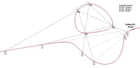
1. Cotterill’s Point of P1 through P4 is P1+P2+P3+P4 – N, abbreviated as (PP4–N).
2. The Cayley-Bacharach point of P1 through P8 is (3N-PP8).
3. The 7P-pivot.

1.  Cotterill’s Point

Cotterill’s Point of P1, P2, P3, P4 is (P1 . P2) . (P3 . P4).

It is also equal to (P1 . P3) . (P2 . P4), and to (P1 . P4) . (P2 . P3), making it a special point.

Using the point-value rules (especially rule 6), we find:

• (P1 . P2) . (P3.P4) = N – (N – P1 – P2) – (N – P3 – P4) = P1 + P2 + P3 + P4 – N
• (P1 . P3) . (P2.P4) = N – (N – P1 – P3) – (N – P2 – P4) = P1 + P2 + P3+ P4 – N
• (P1 . P4) . (P2.P3) = N – (N – P1 – P4) – (N – P2 – P3) = P1 + P2 + P3+ P4 – N

This conforms that all three constructions yield the same point-values, this proves the existence of a unique point – Cotterill’s Point.

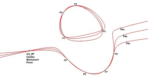
 2.  Cayley-Bacharach point

Cayley-Bacharachs Theorem states that if P1 through P8 lie on a cubic, then every other cubic passing through these eight points also passes through a common ninth point.

The 9^th point is the Cayley-Bacharach Point of the eight.

Define CB9 =be the Cayley-Bacharach Point of P1 through P8.

From rule 8: P1 + P2 + … + P8 + CB9 = 3N.

So: CB9 = 3N – PP8.

This leads to a construction method:

CB9 = (P1 . P2) . (P3 . P4) . (P5 . P6) . (P7 . P8)

Here, Pi . Pj means the third intersection point of CU and line PiPj”.

Using rule 6, this construction confirms CB9 = 3N – PP8.

Any permutation of the eight points yields the same CB9, proving its uniqueness.

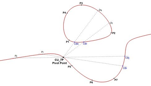
 3.  The 7P-Pivot

Let P1 through P7 be fixed reference points on CU. L

et Px and Py be two additional random points on CU.

Each set of eight points define a Cayley-Bacharach Point:

• CBx for (P1, …, P7, Px)
• CBy for (P1, …, P7, Py)

Their intersection point lies on CU and turns out to be a fixed point—the 7P-Pivot.

This point was contributed by Eckart Schmidt.

Proof

Recall:

• Pi.Pj = (Pi + Pj) – N
• CBi = 3N – (PP9 – Pi)

Let:

• Tx = Px . CBx, then Tx = (Px + (3N – (PP7 + Px)) – N) = 2N – PP7
• Ty = Py . CBy, then Ty = (Py + (3N – (PP7 + Py)) – N) = 2N – PP7

Both Tx and Ty are constructed both as points on CU and have the same value: 2N – PP7.

Since Px and Py do not appear in the final expression, the point is independent of them.

Thus, the 7P-Pivot is a unique point on CU determined solely by the seven reference points.

Estimated human page views: 8