CU-Sx1 The CU-Cayleyan
The Cayleyan and Its Geometric Context
The Hessian is the locus of points P for which the P-Polar Conic degenerates into 2 straight lines.
The Cayleyan (sometimes spelled Cayleyian) is the envelope of these degenerate lines – a curve formed by their continuous variation.
Concepts used
The following notions will be referenced throughout this discussion:
- The Reference Cubic CU
- The Cayleyan CAY of CU: CU-Sx1
- The Hessian HE of CU: CU-Cu1
- The Harmonic Polars of CU: CU-9L1
- The Polar Conic of a point P with respect to CU: CU-P-Co1
- The 4 Poles of a line L with respect to CU: CU-L-4P1
- The Quadri-Pole of a line L: QA-Tf10(L)
Properties of the Cayleyan
- The Cayleyan is a sextic curve—a curve of degree 6.
- This means that any line in the plane will intersect the Cayleyan in exactly six points, which may be real or imaginary.
- The Cayleyan is also of class 3.
- This implies that from any point in the plane, there exist exactly three tangents to the Cayleyan, again possibly imaginary.
CU-Cayleyan-14-plus-Hessian-F-Tangents-Polars.fig
Additional properties
Furthermore the Cayleyan is:
1) The envelope of all lines through 2 corresponding points of the Hessian. These corresponing points (H1,H2) of the Hessian HE are some point H1 on HE and the intersection point H2 of the straight lines of the degenerated H1-Polar Conic wrt Reference Cubic CU.
2) The envelope all lines forming the degenerated Polar Conics of points of the Hessian
(these 2 definitions are equivalent)
3) The locus of the contact point of the line with the curve, which is the harmonic conjugate of the complementary point wrt the 2 corresponding points.
For further clarification of the terms corresponding points and complementary point, see:
Classical Description by Durège
The most concise description of the Cayleyan comes from Durège. See [84], page 264.
He writes:
498. Lässt man eine Gerade G alle möglichen Lagen in der Ebene annehmen
und bestimmt jedesmal ihre vier Pole a b c d bezüglich einer Curve 3. O.,
so beschreiben die Diagonalpunkte des vollständigen Vierecks a b c d
die Hesse’sche Curve und die Seiten dieses Vierecks hüllen die Cayley’sche Curve ein.
– Denn diese Seiten bilden die sämmtlichen conischen Polaren, welche aus Geradenpaaren bestehen.
Translation:
498. Consider a line G at all possible positions in the plane
and determine its four poles a b c d with respect to a curve of the 3rd degree,
then the diagonal points of the complete quadrangle a b c d will describe
the Hessian Curve and the sides of this quadrangle will envelope the Cayleyan Curve.
Because of these sides forming all the polar conics, which consist of pairs of straight lines.
The four poles of a line like described by Durège are CU-L-4P1.
Summary
- All P-Polar Conics wrt CU will intersect in 4 common fixed points, when P is a point on some fixed line L in the plane.
- These 4 common fixed points are called the 4 poles of L wrt CU.
- The Hessian is the locus of points P where the P-Polar Conics wrt CU degenerates into 2 lines.
- The Cayleyan is the curve enveloped by these straight lines.
Construction
- Given Reference Cubic CU.
- Choose 3 random points P, Q, R (not necessary lying on CU) such that their Polar Conics mutually intersect in 4 real points.
- These three polar conics will intersect mutually in 3 distinct sets of 4 points each. Thus, we obtain 3 quadrangles QA’s. For the construction, only two of these QA’s are needed.
- For each QA (quadrangle), apply the QA-Tf10 transformation *) to map the 6 QA-sides to 6 points Ti. Two QA’s yield a total of 2×6 points Ti.
- As the reference QA, just any 4 reference points mat be selected.
- Construct a cubic CUx that passes through 9 of the 12 points Ti. It will then be observed that the remaining 3 points Ti also lie on this cubic CUx.
- Choose a variable point X on the constructed cubic Cux and draw the tangent Tx to Cux at point X.
- Map Tx the QA-Tf10 transformation *) into point Px.
- The locus of Px traces out the Cayleyan.
See reference: QPG#2160.
Note
*) Since any Reference Quadrangle can be chosen fot the QA-Tf10 transformation, a convenient choice for barycentric coordinatecal culations is the quadrangle with vertices (1:0:0), (0:1:0), (0:0:1), and (p:q:r).
In this case QA-Tf10 [(p:q:r)] = (2p+q+r : p+2q+r : p+q+2r).
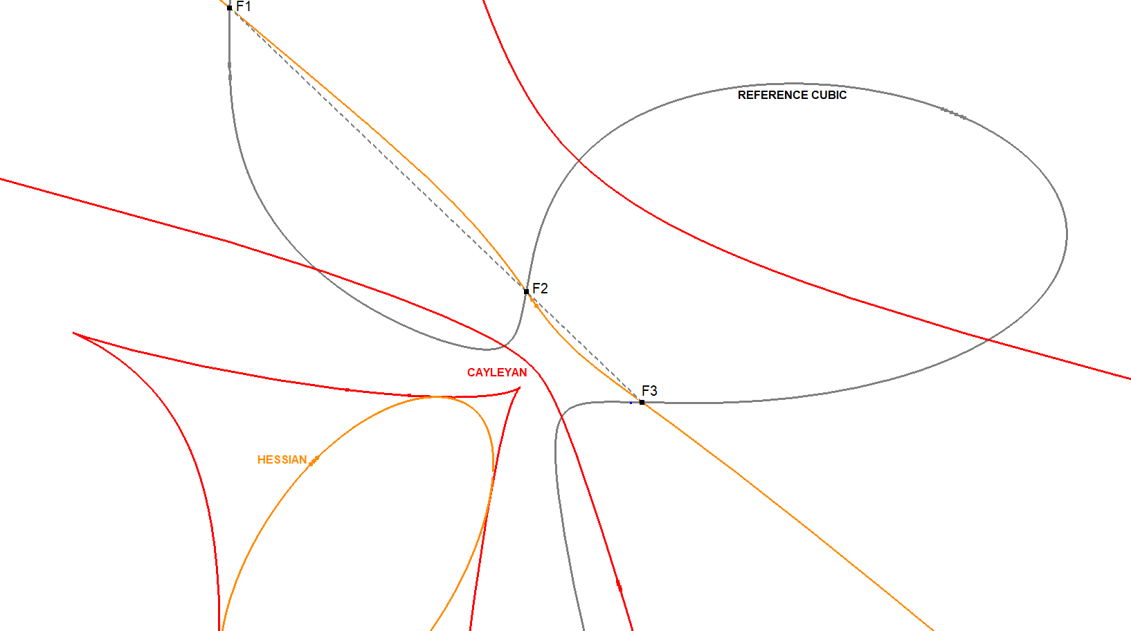
CU-Cayleyan-16-plus-Hessian-F-Tangents-Polars.fig
The Reference Cubic CU, the Hessian HE and the Cayleyan CAY are intricately connected in several geometric ways.
Intersection of CU and HE
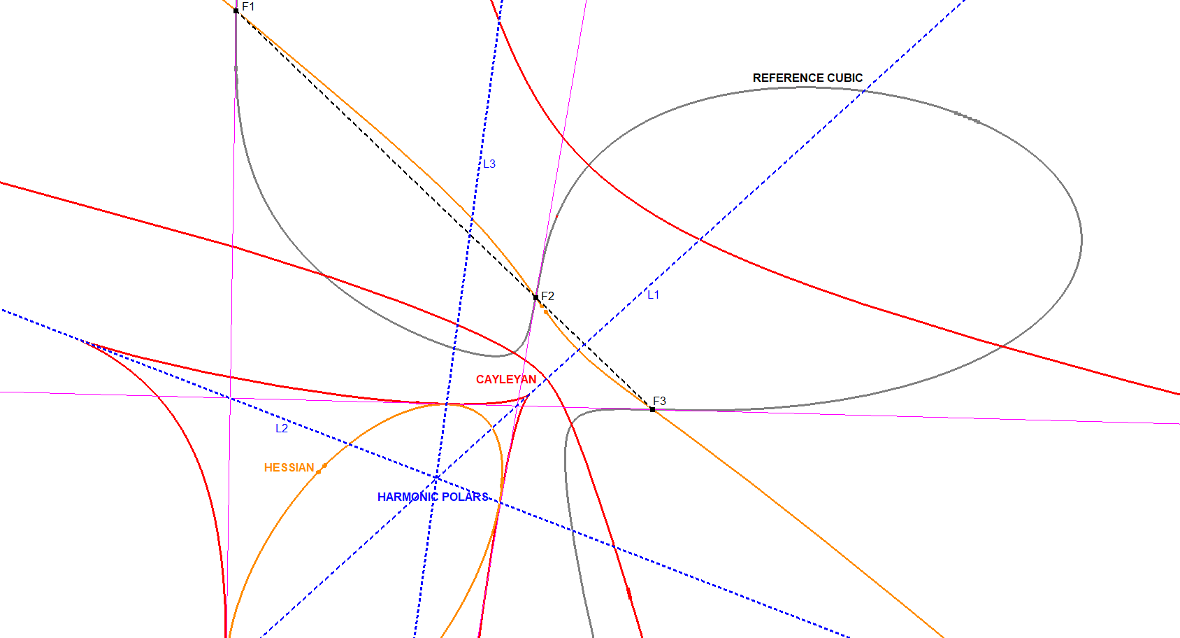
As shown in the image above, CU and HE intersect in 3 real Flexpoints F1, F2, F3, which lie on a straight line (see CU-9P1).
The tangents to CU at these points are also tangent to CAY and HE at the same locations. These points are where the Harmonic Polars Li and the Fi-Tangents converge.
Intersection of CU and CAY
In the next image, CU and CAY intersect in 6 real points.
The tangents to CU at these points are also tangent to HE, per pair of tangents intersects on a harmonic polar (see CU-9L2).
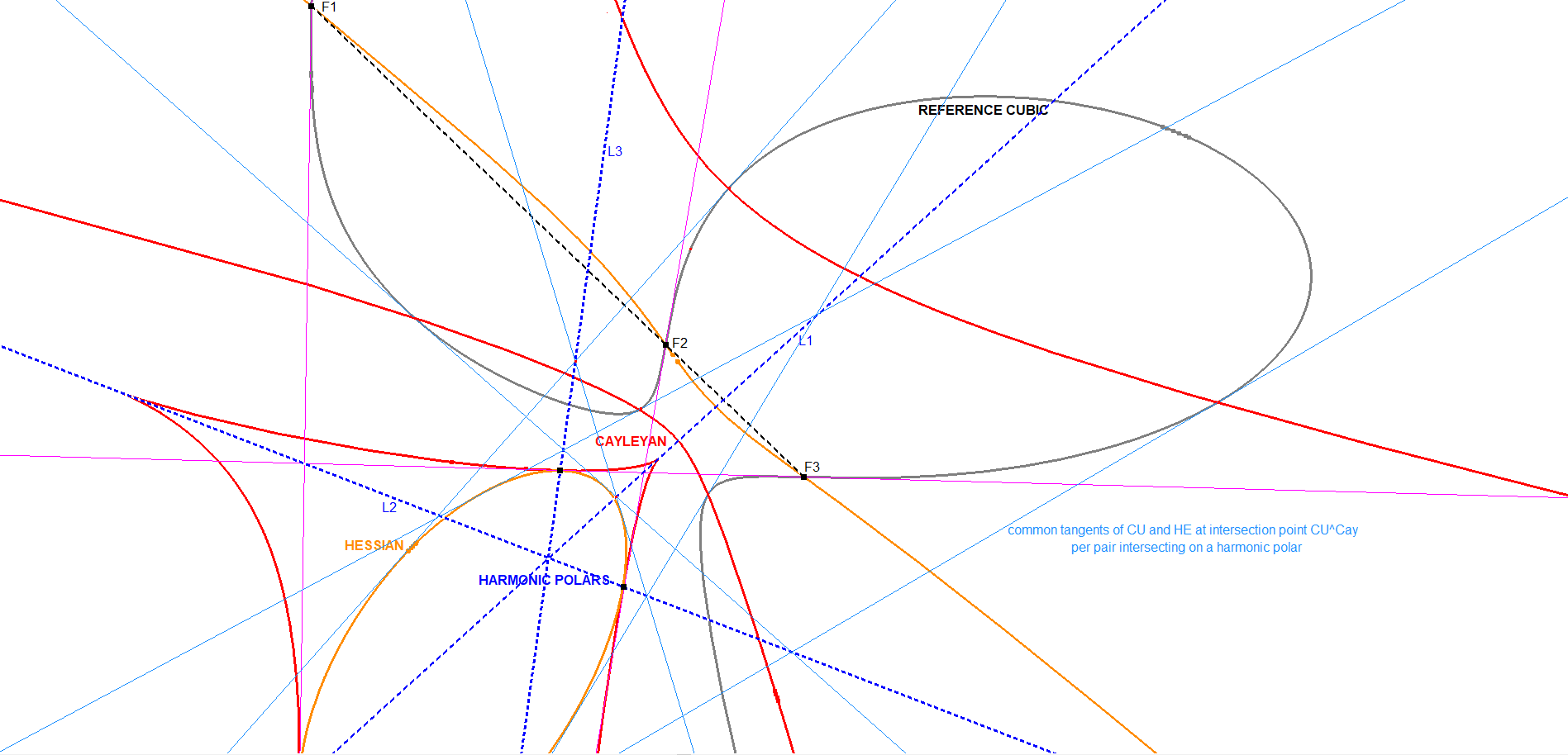
CU-Cayleyan-17-plus-Hessian-F-Tangents-Polars.fig
Further reading
More information about the Cayleyan can be found in:
- CU-5
- [66], QPG messages #2108, #2118-2121, #2124, #2128, #2137, #2156, #2160, #2163-2169
- Literature:
Estimated human page views: 155