QL-Tf3: CSCe-Transformation
The CSCe Transformation is a linear transformation mapping lines into points.
Consequently its inverse transformation, here called QL-Tf3R or CSCeR, is also a linear transformation mapping points into lines.
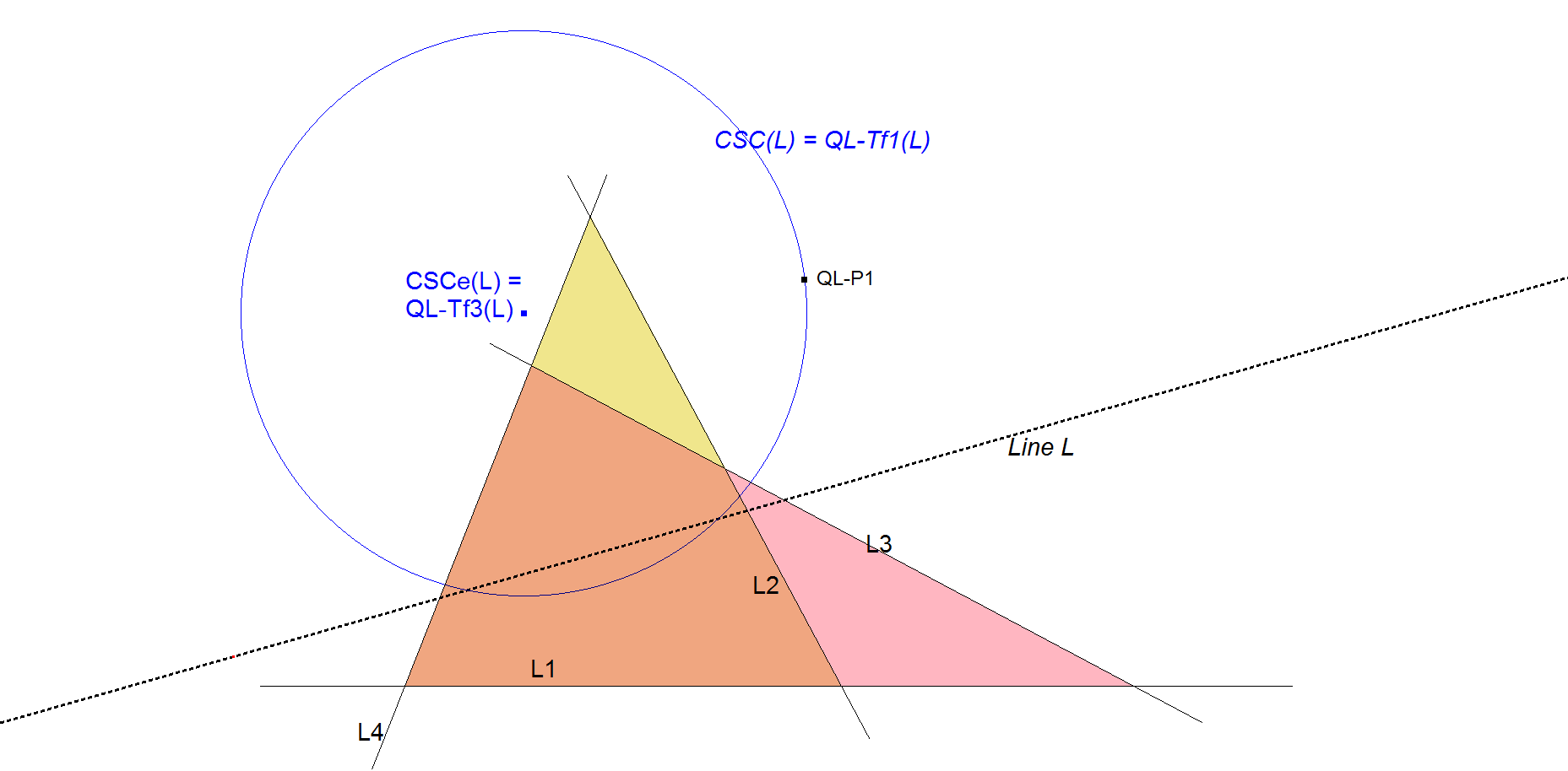
This transformation is related to QL-Tf1 (Clawson-Schmidt Conjugate), often abbreviated with CSC. CSC transforms lines into “circles-through-QL-P1” and transforms “circles-through-QL-P1” into lines. CSCe is transforming a line into the center of the “circle-through-QL-P1”.
CSCe was introduced in [34], QFG-message #430.
Special about this transformation is this property:
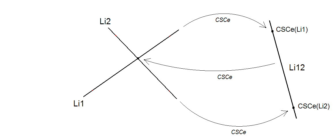
Let Li1 and Li2 be two random lines.
Let Li12 be new line CSCe(n1).CSCe(n2).
Now CSCe(Li12) will be Li1^Li2.
A corresponding property is valid for CSCeR.
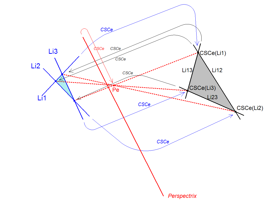
The transformation CSCe even becomes more beautiful when dealing with 3 random lines:
- Let Li1, Li2 and Li3 be three random lines.
- Let Tr1 = Triangle (Li1,Li2,Li3) and Tr2 = Triangle (CSCe(Li1), CSCe(Li2), CSCe(n3)).
- Now each vertex or line from these triangles will be mutually related by CSCe or CSCeR. When transforming a triangle the vertices or the sidelines can be transformed (resp. by CSCeR and CSCe), the outcome will be the same transformed triangle!
- And Tr1 will be perspective with Tr2 with some perspector Pe and some perspectrix Px.
- Moreover CSCe(Px) = Pe and correspondingly CSCeR(Pe) = Px.
- Another consequence is that every QL-Triangle can be transformed into a point Pe and line Px (using CSCe or CSCeR). This can be considered as another QL-transformation mapping a QL-Triangle into a QL-point and a QL-line.
Corresponding properties are valid for CSCeR.
Consequently CSCe and CSCeR have a Dual-function, meaning:
Each line has a corresponding point and each point has a corresponding line.
Lines are transformed into points and points into lines.
The Trilinear Pole and the Trilinear Polar have corresponding functions in a triangle.
These special properties occur when the transformation is an involutary correlation or also called a polarity.
See [53], page 61.
This can be checked in the transformation matrix in general form:
| a11 | a12 | a13 |
| a21 | a22 | a23 |
| a31 | a32 | a33 |
when the matrix equals its transpose matrix meaning that a12=a21, a23=a32, a13=a31.
See [54], page 80, section 3.4.
For QL-Tf3 this is true as can be deducted from following transformed coordinates.
More information about QL-Tf3 can be found at [34], QFG-messages #430, #435, #436, #442, #453, #454, #456, #465, #470, #471, #480, #489, #492, #1682, #1684, #1687, #1691, #1697.
CT-coordinates of the CSCe Transformation of some line (x:y:z)
(-a2 m n (a4 l2 – a2 b2 l2 – a2 c2 l2 – a4 l m + a2 b2 l m + 2 a2 c2 l m + b2 c2 l m – c4 l m – a4 l n + 2 a2 b2 l n – b4 l n + a2 c2 l n + b2 c2 l n + a4 m n – 2 a2 b2 m n + b4 m n – 2 a2 c2 m n – 2 b2 c2 m n + c4 m n) x
– a2 b2 l m n (-a2 l + b2 l – c2 l + a2 m – b2 m – c2 m + 2 c2 n) y
– a2 c2 l m n (-a2 l – b2 l + c2 l + 2 b2 m + a2 n – b2 n – c2 n) z :
-a2 b2 l m n (-a2 l + b2 l – c2 l + a2 m – b2 m – c2 m + 2 c2 n) x –
b2 l n (a2 b2 l m – b4 l m + a2 c2 l m + 2 b2 c2 l m – c4 l m – a2 b2 m2 + b4 m2 – b2 c2 m2 + a4 l n – 2 a2 b2 l n + b4 l n – 2 a2 c2 l n – 2 b2 c2 l n + c4 l n – a4 m n + 2 a2 b2 m n – b4 m n + a2 c2 m n + b2 c2 m n) y –
b2 c2 l m n (2 a2 l – a2 m – b2 m + c2 m – a2 n + b2 n – c2 n) z :
-a2 c2 l m n ( -a2 l – b2 l + c2 l + 2 b2 m + a2 n – b2 n – c2 n) x –
b2 c2 l m n (2 a2 l – a2 m – b2 m + c2 m – a2 n + b2 n – c2 n) y –
c2 l m (a4 l m – 2 a2 b2 l m + b4 l m – 2 a2 c2 l m – 2 b2 c2 l m + c4 l m + a2 b2 l n – b4 l n + a2 c2 l n + 2 b2 c2 l n – c4 l n – a4 m n + a2 b2 m n + 2 a2 c2 m n + b2 c2 m n – c4 m n – a2 c2 n2 – b2 c2 n2 + c4 n2) z )
CT-coordinates of the Inverse CSCe Transformation CSCeR of some point (x:y:z)
(b2 c2 l (-a2 b2 l2 m2 + b4 l2 m2 – a2 c2 l2 m2 – 2 b2 c2 l2 m2 + c4 l2 m2 + a2 b2 l m3 – b4 l m3 + b2 c2 l m3 – a4 l2 m n + 2 a2 b2 l2 m n – 2 b4 l2 m n + 2 a2 c2 l2 m n + 4 b2 c2 l2 m n – 2 c4 l2 m n + a4 l m2 n – a2 b2 l m2 n + 2 b4 l m2 n – b2 c2 l m2 n – c4 l m2 n – a2 b2 m3 n – a2 b2 l2 n2 + b4 l2 n2 – a2 c2 l2 n2 – 2 b2 c2 l2 n2 + c4 l2 n2 + a4 l m n2 – b4 l m n2 – a2 c2 l m n2 – b2 c2 l m n2 + 2 c4 l m n2 – a4 m2 n2 + a2 b2 m2 n2 + a2 c2 m2 n2 + a2 c2 l n3 + b2 c2 l n3 – c4 l n3 – a2 c2 m n3) x
+ a2 b2 c2 l m (-a2 l2 m + b2 l2 m – c2 l2 m + a2 l m2 – b2 l m2 – c2 l m2 – b2 l2 n + c2 l2 n + a2 l m n + b2 l m n + 3 c2 l m n – a2 m2 n + c2 m2 n – 2 c2 l n2 – 2 c2 m n2 + c2 n3) y
+ a2 b2 c2 l n (b2 l2 m – c2 l2 m – 2 b2 l m2 + b2 m3 – a2 l2 n – b2 l2 n + c2 l2 n + a2 l m n + 3 b2 l m n + c2 l m n – 2 b2 m2 n + a2 l n2 – b2 l n2 – c2 l n2 – a2 m n2 + b2 m n2) z :
a2 b2 c2 l m (-a2 l2 m + b2 l2 m – c2 l2 m + a2 l m2 – b2 l m2 – c2 l m2 – b2 l2 n + c2 l2 n + a2 l m n + b2 l m n + 3 c2 l m n – a2 m2 n + c2 m2 n – 2 c2 l n2 – 2 c2 m n2 + c2 n3) x
+ a2 c2 m (-a4 l3 m + a2 b2 l3 m + a2 c2 l3 m + a4 l2 m2 – a2 b2 l2 m2 – 2 a2 c2 l2 m2 – b2 c2 l2 m2 + c4 l2 m2 – a2 b2 l3 n + 2 a4 l2 m n – a2 b2 l2 m n + b4 l2 m n – a2 c2 l2 m n – c4 l2 m n – 2 a4 l m2 n + 2 a2 b2 l m2 n – b4 l m2 n + 4 a2 c2 l m2 n + 2 b2 c2 l m2 n – 2 c4 l m2 n + a2 b2 l2 n2 – b4 l2 n2 + b2 c2 l2 n2 – a4 l m n2 + b4 l m n2 – a2 c2 l m n2 – b2 c2 l m n2 + 2 c4 l m n2 + a4 m2 n2 – a2 b2 m2 n2 – 2 a2 c2 m2 n2 – b2 c2 m2 n2 + c4 m2 n2 – b2 c2 l n3 + a2 c2 m n3 + b2 c2 m n3 – c4 m n3) y
+ a2 b2 c2 m n (a2 l3 – 2 a2 l2 m + a2 l m2 – c2 l m2 – 2 a2 l2 n + 3 a2 l m n + b2 l m n + c2 l m n – a2 m2 n –
b2 m2 n + c2 m2 n + a2 l n2 – b2 l n2 – a2 m n2 + b2 m n2 – c2 m n2) z :
a2 b2 c2 l n (b2 l2 m – c2 l2 m – 2 b2 l m2 + b2 m3 – a2 l2 n – b2 l2 n + c2 l2 n + a2 l m n + 3 b2 l m n + c2 l m n – 2 b2 m2 n + a2 l n2 – b2 l n2 – c2 l n2 – a2 m n2 + b2 m n2) x
+ a2 b2 c2 m n (a2 l3 – 2 a2 l2 m + a2 l m2 – c2 l m2 – 2 a2 l2 n + 3 a2 l m n + b2 l m n + c2 l m n – a2 m2 n – b2 m2 n + c2 m2 n + a2 l n2 – b2 l n2 – a2 m n2 + b2 m n2 – c2 m n2) y
+ a2 b2 n (-a2 c2 l3 m + a2 c2 l2 m2 + b2 c2 l2 m2 – c4 l2 m2 – b2 c2 l m3 – a4 l3 n + a2 b2 l3 n + a2 c2 l3 n + 2 a4 l2 m n – a2 b2 l2 m n – b4 l2 m n – a2 c2 l2 m n + c4 l2 m n – a4 l m2 n – a2 b2 l m2 n + 2 b4 l m2 n – b2 c2 l m2 n + c4 l m2 n + a2 b2 m3 n – b4 m3 n + b2 c2 m3 n + a4 l2 n2 – 2 a2 b2 l2 n2 + b4 l2 n2 – a2 c2 l2 n2 – b2 c2 l2 n2 – 2 a4 l m n2 + 4 a2 b2 l m n2 – 2 b4 l m n2 + 2 a2 c2 l m n2 + 2 b2 c2 l m n2 – c4 l m n2 + a4 m2 n2 – 2 a2 b2 m2 n2 + b4 m2 n2 – a2 c2 m2 n2 – b2 c2 m2 n2) z )
Examples of CSCe Transformations
| Line | Point |
|---|---|
| QL-L2 Steiner Line | QL-P4 |
| QL-L3 Pedal Line | antipode of QL-P1 on QL-Ci3 |
| QL-L5 NSM Line | infinity point of QL-P4.CSCe(QL-L1) |
| QL-P3.QL-P4 | Point on QL-L2 |
Properties
-
- CSCe(QL-P3.QL-P4) is the intersection of QL-L2 and CSC(QL-Ci6). See [34], Eckart Schmidt, message #1687.
- CSC-images of two points and the CSCe-image of lines through the circumcenter of the two points and QL-P1 are collinear:
- If two lines are parallel, their CSCe-images and QL-P1 are collinear:
- If lines have a common point, their CSCe-images are collinear:
- If two lines intersect in P, their CSCe-images and the CSC-images of points on a circle round P through QL-P1 are collinear:
- CSC(CSCe(Line)) = Reflection of QL-P1 in Line (QFG#435).
- CSCeR(QL-Px) = CSCe(line pencil through QL-Px)
Estimated human page views: 993