QL-Tf1: Clawson-Schmidt Conjugate
The Clawson-Schmidt Conjugate of a point P is a transformation of a point P in such a way that each defining line of the Reference Quadrilateral is transformed in the circumcircle of the triangle formed by the other 3 lines of the Reference Quadrilateral.
It is a conjugate because applying two times this transformation ends up in the original point.
The transformation is often abbreviated as CSC.
Origin of the conjugate
John Wentworth Clawson suggested an inversion transformation wrt some circle with the Miquel point as center (see [22] and [40]). It was Eckart Schmidt who gave a very useful form to this inversion by modifying it in this way:
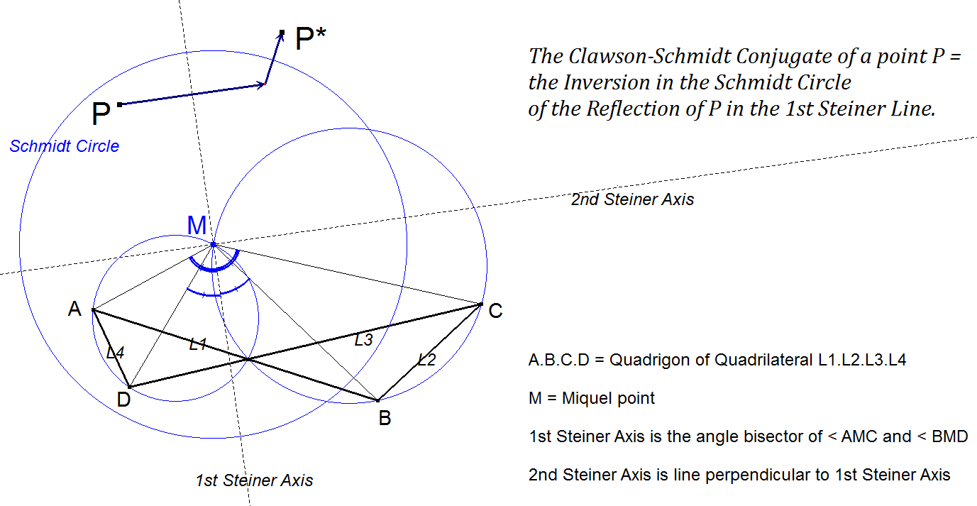
In each quadrigon of a quadrilateral we have 4 points A, B, C, D in this order. Let M be the Miquel Point. Now the Angle Bisectors of <AMC and of <BMD are the same line. See [15d]. Moreover this line is the same (invariant) for each QL-Quadrigon. Let this line be called the 1st Steiner Axis. Let the 2nd Steiner Axis be the line perpendicular at the 1st Steiner Line in M.
Let the circle with Circumcenter M and with radius = √[MA.MC] = √[MB.MD] be called the Schmidt Circle.
The Clawson-Schmidt Conjugate of a point P is the Inversion wrt the Schmidt Circle of the Reflection in the 1st Steiner Axis.
Moreover the reflection and inversion can be performed in reversed order.
The result is a conjugation that transforms each defining line of the Reference Quadrilateral into the circumcircle of the triangle formed by the other 3 lines of the Reference Quadrilateral.
Relationship with Steiner-rules
The 1st and 2nd Steiner-Axes are described in the Steiner rules (8) and (9). That’s why they are named after Steiner.
Rules 8, 9, 10 of Steiner about quadrilaterals state (see [4]):
(8) Each of the four possible triangles in a quadrilateral has an incircle and three excircles.
The centers of these 16 circles lie, four by four, on eight new circles.
(9) These eight new circles form two sets of four, each circle of one set being orthogonal to each circle of the other set.
The centers of the circles of each set lie on a same line.
These two lines are perpendicular.
(10) Finally, these last two lines intersect at the point F (Miquel Point).
Both sets of 4 circles as described in (9) are coaxal. One set has an axis with real intersection points of the 4 circles, the other set has an axis with imaginary intersection points of the 4 circles. These axes are called the 1st Steiner-axis (axis with 2 real common intersection points of 4 circles) and the 2nd Steiner-axis (axis with 2 imaginary common intersection points of 4 circles). The common intersection points on the 1st Steiner Axis are the only points in the real plane that are invariant under Clawson-Schmidt Conjugation. See [15d].
The Steiner Axes also can be constructed as the angle bisectors of QL-P1.QL-P4 and the axis of the inscribed Parabola QL-Co1. See [34], Eckart Schmidt, QFG #914.
Construction
Eckart Schmidt describes this construction in [15d]:
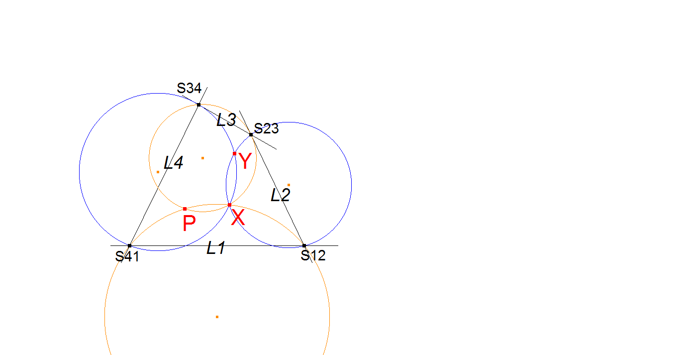
- Choose one Quadrigon of the Reference Quadrilateral. For example S41.S12.S23.S34, where Sij = Intersection Li ^ Lj.
- Let P be a random point. Draw a circle Ci1 through P and the 2 vertices on a side L1 of the Quadrigon. Draw a circle Ci2 through P and the 2 vertices on the opposite side L3 of the Quadrigon. Let X be the 2nd intersection point of Ci1 and Ci2.
- Draw a circle Ci3 through X and the 2 vertices on a third side L2 of the Quadrigon. Draw a circle Ci4 through X and the 2 vertices on the last side L4 of the Quadrigon. Let Y be the 2nd intersection point of Ci3 and Ci4.
- Y is the Clawson-Schmidt Conjugate.
Coordinates:
Let Q (u : v : w) be a random point not on one of the defining lines of the Reference Quadrilateral.
The Clawson-Schmidt Conjugate in CT-coordinates gives this result:
(a2 m n (a2 (l-m) ( l – n) v w + c2 (l – n) v (l u+m v+m w) + b2 (l – m) w ( l u +n v+n w)) :
b2 l n (b2 (m-l) (m-n) u w + c2 (m-n) u (l u+m v+ l w) + a2 (m – l) w (n u+m v+n w)) :
c2 l m (c2 (n – l) (n-m) u v + b2 (n-m) u (l u+ l v + n w) + a2 (n – l) v (m u+m v+n w)))
The Clawson-Schmidt Conjugate in DT-coordinates gives this result:
(b4 L N u (u + v – w) + c4 L M u (u – v + w) – a4 M N u (u + v + w) – 2 b2 c2 L u (N v + M w)
+ 2 a2 b2 N ((u + v) (N2 u + M2 v) – N2 w2) – 2 a2 c2 M (-M2 v2 + (u + w) (M2 u + N2 w)) :
a4 M N v (u + v – w) + c4 L M v (-u + v + w) – b4 L N v (u + v + w) – 2 a2 c2 M v (N u + L w)
– 2 a2 b2 N ((u + v) (L2 u + N2 v) – N2 w2) + 2 b2 c2 L (-L2 u2 + (v + w) (L2 v + N2 w)) :
– 2 a2 b2 N (M u + L v) w + a4 M N w (u – v + w) + b4 L N w (-u + v + w) – c4 L M w (u + v + w)
– 2 b2 c2 L (-L2 u2 + (v + w) (M2 v + L2 w)) + 2 a2 c2 M (-M2 v2 + (u + w) (L2 u + M2 w)))
where:
L = m2 – n2 M = n2 – l2 N = l2 – m2
If we take the Miquel triangle as reference triangle ABC (C in the Miquel Point), then the Clawson-Schmidt Conjugate QL-Tf1 gets a very simple form for Quadrigons:
(x : y : z) -> (-a2 y : -b2 x : (a2 y z+b2 z x+c2 x y) / (x+y+z)).
Let L3^L4 = P4 = (u : v : w), then:
L2^L3 = P3 = (a2 w : T : c2 u),
L1^L2 = P2 = (a2 v : b2 u : T),
L4^L1 = P1 = (T : b2 w : c2 v)
where T = -(a2 v w+b2 w u+c2 u v) / (u+v+w).
See [34], QFG # 338 by Eckart Schmidt.
Examples of Clawson-Schmidt Conjugates
| Point/Line/Curve –1 | Point/Line/Curve –2 |
|---|---|
| General | |
| Defining Quadrilateral Lines: L1, L2, L3, L4 | Circumcircle of corresponding QL-Component Triangle |
| Intersection point Li ^ Lj | Opposite intersection point Lk ^ Ll |
| A line not through QL-P1 | A circle through QL-P1 |
| A line through QL-P1 | A line through QL-P1 |
| A circle with QL-P1 as center | Another circle with QL-P1 as center |
| Points/Lines/Curves | |
| QL-P1: Miquel Point | Some (undefined) point at infinity |
| QL-P4: Miquel Circumcenter | Reflection of QL-P1 in QL-L2 (Steiner Line) |
| QL-L2 Steiner Line | QL-Ci3 Miquel Circle |
| QL-Co1: Inscribed Parabola | QL-Qu1: Morley’s Mono QL-Cardioid |
| Circle through X(186) points in QL-CT’s See QL-P28, center of this circle. |
Circle through X(265) points in QL-CT’s See QL-P29, center of this circle. |
| QG-P1: Diagonal Crosspoint | QA-P4: Isogonal Center |
| QG-P17: Projection QG-P1 on QG-L1 | QG-P18: Quasi Isogonal Crosspoint |
| QG-L1: 3rd Diagonal | QG-Ci3: Quasi Isogonal Circle |
| QA-Ci1: QA-Circumcircle DiagonalTriangle | Circle through QG-2P2a, QG-2P2b, QA-P4, QG-P19 |
| Invariances | |
| Steiner Bisector Circle-i (i=1–8) (circles in rule 9 of Steiner) |
Same Steiner Bisector Circle-i (i=1–8) |
| Schmidt Circle | Schmidt Circle |
| Intersection point 1st Steiner-Axis ^ Schmidt Circle |
Same intersection point 1st Steiner-Axis ^ Schmidt Circle (the only invariant points there are) |
| Intersection point 2nd Steiner-Axis ^ Schmidt Circle |
Other intersection point 2nd Steiner-Axis ^ Schmidt Circle (switching points) |
| QL-Cu1: Quasi Isogonal Cubic | QL-Cu1: Quasi Isogonal Cubic |
Performances in Quadrangles
There are special surprises applying the Clawson-Schmidt Conjugate wrt Quadrangles:
- QL-Tf1 produces at Quadrigon-level using QG-P1 (the Diagonal Crosspoint) a Quadrangle-Point: QA-P4 (Isogonal Center) which is valid for all its QA-Quadrigons. See [15d].
- QL-Tf1 produces at Quadrigon-level using QG-P16 (the Schmidt Point) a Quadrangle-Point: QA-P3 (Gergonne-Steiner Point) which is valid for all its QA-Quadrigons (Eckart Schmidt, November 26, 2012).
- Consider the 4 points of a QL-Quadrigon as a QA-Quadrigon also defining a Quadrangle. Let M2 and M3 be the Miquel Points of the other two QA-Quadrigons. Now M2 and M3 are mutual Clawson-Schmidt Conjugates wrt the 1st QA-Quadrigon. See [15b] and [15d].
- For a Quadrangle there are three Clawson-Schmidt Conjugates wrt the quadrilaterals
- P1P2, P2P3, P3P4, P4P1 (CSCa),
- P1P2, P2P4, P4P3, P3P1 (CSCb),
- P1P4, P4P2, P2P3, P3P1 (CSCc).
- Now the product of two of these conjugates achieves the third one. The product of all three achieves the identity. See [15d]. The QA-DT-P4 Cubic (QA-Cu1) of the quadrangle is invariant under these three transformations.
- Let P be some point on the QA-DT-P4 Cubic (QA-Cu1) and let Pa = CSCa(P), Pb = CSCb(P), Pc = CSCc(P). The tangents at P, Pa, Pb, Pc to the cubic QA-Cu1 coincide in the Isogonal Center (QA-P4) of the Quadrangle P.Pa.Pb.Pc. See [15b].
Properties
- The intersections of lines L through P and the tangents T at the QL-Tf1-image-circle of L in QL-P1 give an orthogonal hyperbola, centered in the midpoint of P.QL-P1 with asymptotes parallel to the Steiner axes. See [34], Eckart Schmidt, QFG-message #1666.
- Let Q2 be the midpoint of QL-P1 and random point Q1. Now QL-Tf1[Q1) will be the midpoint of QL-P1 and QL-Tf1(Q2). See [34], QFG-message #1689.
- Let Q2 be a point collinear with QL-P1 and random point Q1 (consequently QL-P1, QL-Tf1(Q1) and QL-Tf1(Q2) will be collinear too). Now Q1.QL-Tf1(Q2) will be parallel to Q2.QL-Tf1(Q1). See [34], QFG-message #1689.
- Denote QL-Tf1a=QL-Tf1 applied in 1st QA-Quadrigon, QL-Tf1b=QL-Tf1 applied in 2nd QA-Quadrigon, QL-Tf1c=QL-Tf1 applied in 3rd QA-Quadrigon. QL-Tf1a(QL-Tf1b(QL-Tf1c(P))) = P. The 3 versions of QL-Tf1 in a Quadrangle applied in any order.
Estimated human page views: 1526